Amor (Neo) 2017 BR93

This NEO is listed in the page of Asteroids with Comet-Like Orbits maintained by Y. Fernandez.

I simulated 100 clones of this asteroid in the past 10^8 days trying to confirm its possible cometary origin: the goal is to determine whether some clones might have arrived from the outskirt of the solar system - arbitrary threshold: 100 AU.

The first step was to generate clones having orbital parameters distributed around the nominal ones with 1-sigma uncertainty as follows:

JPL Small-Body Database Browser

 

(2017 BR93)

Classification: Amor [NEO]          SPK-ID: 3767926

[ Ephemeris | Orbit Diagram | Orbital Elements | Physical Parameters | Close-Approach Data ]

[ show orbit diagram ]

Orbital Elements at Epoch 2458000.5 (2017-Sep-04.0) TDB Reference: JPL 5 (heliocentric ecliptic J2000)  Element Value Uncertainty (1-sigma)   Units  e .7217412317070279 0.0001002 a 4.142675777273991 0.0015088 au q 1.152735859221392 3.3533e-05 au i 15.35366999553024 0.001219 deg node 97.57957971696266 0.0028893 deg peri 318.8120872155768 0.0036121 deg M 38.89039107061564 0.021706 deg tp 2457667.794750083124 (2016-Oct-06.29475008) 0.0066681 JED period 3079.781063466159 8.43 1.6825 0.004606 d yr n .1168914259102677 6.3858e-05 deg/d Q 7.13261569532659 0.0025977 au

Orbit Determination Parameters    # obs. used (total)      34      data-arc span      75 days      first obs. used      2016-11-23      last obs. used      2017-02-06      planetary ephem.      DE431      SB-pert. ephem.      SB431-N16      condition code      6      fit RMS      .44498      data source      ORB      producer      Otto Matic      solution date      2017-Nov-30 06:50:30   Additional Information  Earth MOID = .222957 au   Jupiter MOID = .227161 au   T_jup = 2.447

The orbit condition code is 6 so there is still a lot of uncertainty.

Simulation approach

Mercury6 Integrator

reference:

J.E.Chambers (1999) 

A Hybrid Symplectic Integrator that Permits Close Encounters between Massive Bodies''. Monthly Notices of the Royal Astronomical Society, vol 304, pp793-799.

           Integration parameters
           ----------------------

   Algorithm: Bulirsch-Stoer (conservative systems)

   Integration start epoch:         2458000.5000000 days
   Integration stop  epoch:      -100000000.0000000
   Output interval:                     100.000
   Output precision:                 medium

   Initial timestep:                0.050 days
   Accuracy parameter:              1.0000E-12
   Central mass:                    1.0000E+00 solar masses
   J_2:                              0.0000E+00
   J_4:                              0.0000E+00
   J_6:                              0.0000E+00
   Ejection distance:               1.0000E+02 AU
   Radius of central body:          5.0000E-03 AU


Simulation Results

• 75 out of 100 clones have a cometary like orbit.
• of which: 16 came on a hyperbolic orbit. The one that had the highest speed had a Vinfinity about 15.2 km/s (Vinfinity = 42.1219*sqrt(-0.5/a) --> the semi-major axis being about -3.82 AU

The time (Year) when they entered the solar system was distributed as follows:

   Min. 1st Qu.  Median    Mean 3rd Qu.    Max.
-276249 -148774  -75459  -98680  -33904    -709

In a graphical form:

A look at the nominal asteroid

The nominal asteroid itself does not have a cometary origin in the last 10^8 days. It appears to be nevertheless on a unstable orbit, there was a time in the past when its aphelion was at about 70 AU.

In the following plots (made with R package ggplot2), the vertical dashed lines show a close encounter with Jupiter.

A look at the clones - "footprint" diagrams

At any given time in the past, a clone had a certain perihelium q and a certain aphelium Q (I disregard the clones when on an hyperbolic trajectory because Q would be infinite).

Let's imagine that we plot all possible q-Q points in a diagram: the highest density area is the one where the clones happened to be for most of the time.

This is shown here ( I have used the R function stat_density2d):

In the diagram above, we can also see the current q-Q of the asteroid together with that of Jupiter and Saturn.
In a similar way, these are the footprints for w-om and e-i:

 

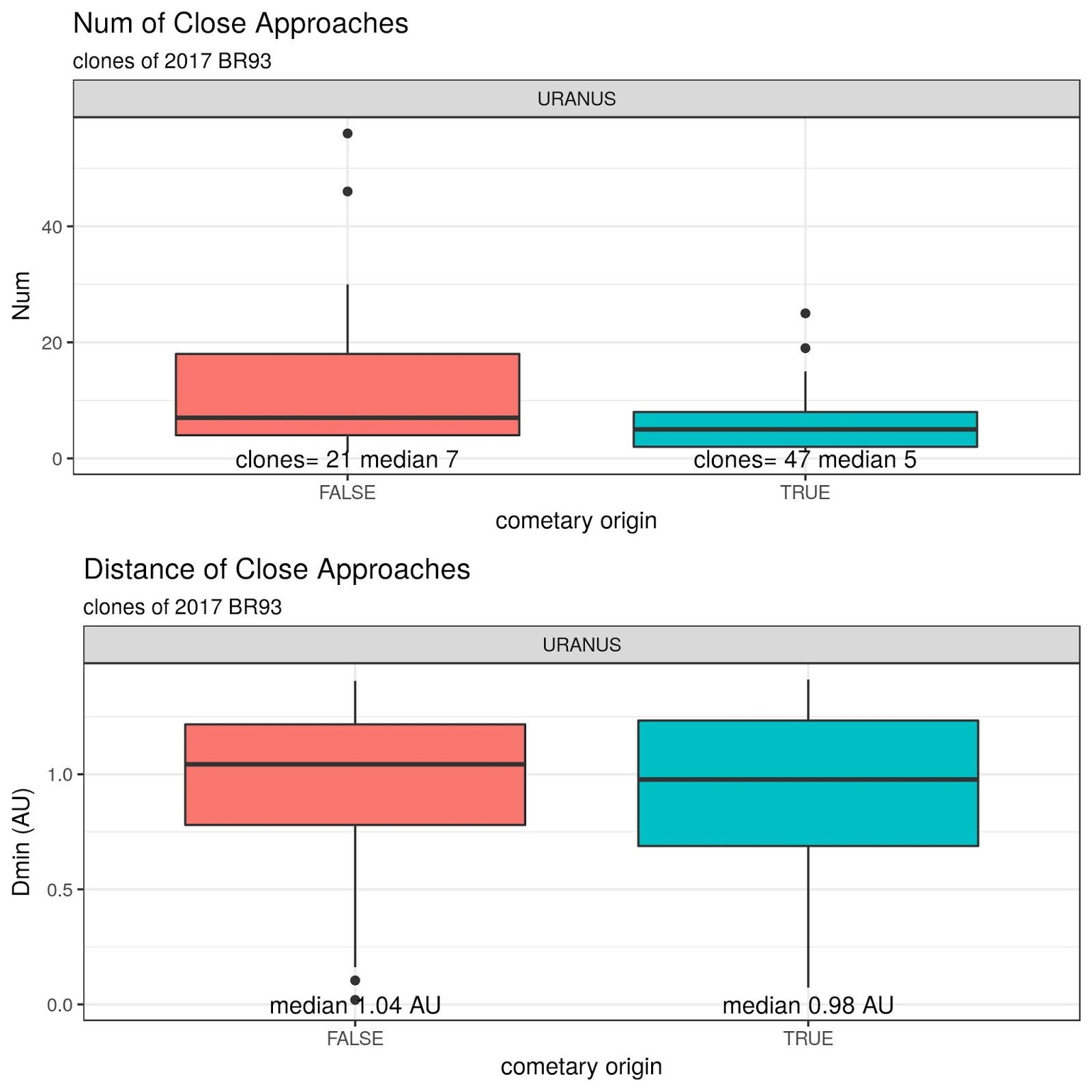
Analysis of close approaches
These plots show the distribution of close appproaches (number and Dmin distance) between the clones and the major planets.

Kind Regards,
Alessandro Odasso

Amor 2002 RN38

This NEO is listed in the page of Asteroids with Comet-Like Orbits maintained by Y. Fernandez.

It was also discussed as an object with a likely cometary origin in some papers, among which I found:

• "On Near-Earth Asteroid Study at Department of  Astronomy, Bandung Institute of Technology" by S. Siregar.
• "Assessing the physical nature of near-Earth asteroids through their dynamical histories" by Julio A. Fernández, Andrea Sosa, Tabaré Gallardo, Jorge N. Gutiérrez.

At the time I made this analysis, this Amor was last observed on November 11th, 2017 and the orbit uncertainty is 0 being based on 119 observations acquired in the last 15 years.

JPL Small-Body Database Browser:

Orbital Elements at Epoch 2458000.5 (2017-Sep-04.0) TDB
Reference: JPL 31 (heliocentric ecliptic J2000)

Element Value Uncertainty (1-sigma)   Units  e .6730769823381273 2.1793e-07 a 3.820825408551513 1.2346e-07 au q 1.249115772522818 7.9678e-07 au i 4.160437503290696 1.756e-05 deg node 296.1904517164833 0.00024613 deg peri 118.6156866423836 0.00026072 deg M 357.1006606538095 3.1062e-05 deg tp 2458022.470035828635 (2017-Sep-25.97003583) 0.00023642 JED period 2727.936248200967 7.47 0.00013222 3.62e-07 d yr n .1319678933983206 6.3964e-09 deg/d Q 6.392535044580208 2.0656e-07 au

Orbit Determination Parameters    # obs. used (total)      119      data-arc span      5568 days (15.24 yr)      first obs. used      2002-08-18      last obs. used      2017-11-15      planetary ephem.      DE431      SB-pert. ephem.      SB431-N16      condition code      0      fit RMS      .55328      data source      ORB      producer      Otto Matic      solution date      2017-Nov-16 07:18:58   Additional Information  Earth MOID = .270556 au   Jupiter MOID = .260678 au   T_jup = 2.626

I simulated 100 clones of this asteroid in the past 10^8 days trying to confirm its possible cometary origin: the goal is to determine whether some clones might have arrived from the outskirt of the solar system - arbitrary threshold: 100 AU.

Simulation approach

Mercury6 Integrator

reference:

J.E.Chambers (1999) 

A Hybrid Symplectic Integrator that Permits Close Encounters between Massive Bodies''. Monthly Notices of the Royal Astronomical Society, vol 304, pp793-799.

           Integration parameters
           ----------------------

   Algorithm: Bulirsch-Stoer (conservative systems)

   Integration start epoch:         2458000.5000000 days
   Integration stop  epoch:      -100000000.0000000
   Output interval:                     100.000
   Output precision:                 medium

   Initial timestep:                0.050 days
   Accuracy parameter:              1.0000E-12
   Central mass:                    1.0000E+00 solar masses
   J_2:                              0.0000E+00
   J_4:                              0.0000E+00
   J_6:                              0.0000E+00
   Ejection distance:               1.0000E+02 AU
   Radius of central body:          5.0000E-03 AU


Simulation Results

• 79 out of 100 clones have a cometary like orbit.
• of which: 13 came on a hyperbolic orbit (Vinfinity = 42.1219*sqrt(-0.5/a) --> the minimum absolute value for semi-major axis a was -17.46 AU -->the maximum value for Vinfinity was 7.14 km/s 
• 1 out of 100 was discarded because "hit" the sun (due to extremely high eccentricity).

The time when they entered the solar system was distributed as follows:

   Min. 1st Qu.  Median    Mean 3rd Qu.    Max.
-272319 -151956  -85380 -100222  -38660    -370

In a graphical form:

The most recent arrival in the solar system could have happened a relatively short time ago compared to other asteroids with a cometary like orbit: year 370 B.C.

A look at the nominal asteroid

The nominal asteroid is one of the 79 clones with a cometary like orbit. It apparently arrived in the solar system about in year 87000 B.C 

In the following plots (made with R package ggplot2), the vertical dashed lines show a close encounter with Jupiter.

Close Approaches analysis
For every given planet, every clone had a certain number of close approaches so we can calculate the mean number of close approaches and the mean number of Dmin (distance of the close approach). Even better, we can print a boxplot showing the distribution of the number of close approaches and their distances.

Kind Regards,
Alessandro Odasso

Asteroid 2017 FW17 - an extinct comet?

Asteroid 2017 FW17 was first observed at Pan-STARRS 1, Haleakala on 2017-03-18.
 

Orbital Elements at Epoch 2457831.5 (2017-Mar-19.0) TDB Reference: JPL 5 (heliocentric ecliptic J2000)  Element Value Uncertainty (1-sigma)   Units  e .3756229227781228 0.020776 a 4.071577338499798 0.075338 au q 2.542199558295334 0.13088 au i 4.36476081532836 0.4957 deg node 353.1159388040458 0.37693 deg peri 206.4444762192174 1.1805 deg M 350.7475904922186 0.39597 deg tp 2457908.624933945908 (2017-Jun-04.12493395) 5.191 JED period 3000.837370760166 8.22 83.288 0.228 d yr n .1199665145161817 0.0033297 deg/d Q 5.600955118704262 0.10364 au

Orbit Determination Parameters    # obs. used (total)      15      data-arc span      8 days      first obs. used      2017-03-18      last obs. used      2017-03-26      planetary ephem.      DE431      SB-pert. ephem.      SB431-N16      condition code      8      fit RMS      .96317      data source      ORB      producer      Otto Matic      solution date      2017-Apr-06 09:58:49   Additional Information  Earth MOID = 1.54121 au   Jupiter MOID = .0287021 au   T_jup = 2.913   JPL covariance   MPC orbit ref: MPEC 2017-FF0

The orbit condition code is 8 so it is extremely uncertain.

The object is interesting because it might have a cometary origin although this is difficult to say given the uncertainty.

I generated 100 clones with orbit parameters average and 1-sigma as shown above and simulated what happened in the last 10^8 days.

Note 1:
thanks to Tony Dunn for a comment that he sent me: if its current nominal orbit is correct, this asteroid is a Hilda with a 3:2 resonance with Jupiter.
But as Tony run it forwards and backwards, it leaves the 3:2 resonance within a few hundred years.
Tony has a online simulator that shows the short term Hilda behaviour .

Note 2:
I used Tony Dunn's simulator to check what happens with asteroid using its nominal parameters.  The likely cometary origin seems confirmed

Simulation set-up

Mercury6 Integrator

reference:

J.E.Chambers (1999) 

A Hybrid Symplectic Integrator that Permits Close Encounters between Massive Bodies''. Monthly Notices of the Royal Astronomical Society, vol 304, pp793-799.

           Integration parameters
           ----------------------

   Algorithm: Bulirsch-Stoer (conservative systems)

   Integration start epoch:         2457831.5000000 days
   Integration stop  epoch:      -100000000.0000000
   Output interval:                     100.000
   Output precision:                 medium

   Initial timestep:                0.050 days
   Accuracy parameter:              1.0000E-12
   Central mass:                    1.0000E+00 solar masses
   J_2:                              0.0000E+00
   J_4:                              0.0000E+00
   J_6:                              0.0000E+00
   Ejection distance:               1.0000E+02 AU
   Radius of central body:          5.0000E-03 AU

Simulation results
The result of the simulation is that 47 out of 100 clones might have arrived in the solar system from a distance greater than 100 AU.
Their arrival time is very much uncertain.
Going back in the past, the first arrival was in year 2075 B.C. while the last arrival was in year 249000 B.C.
This is the distribution of arrival times showing a relative moderate peak about 40000 B.C:

Every clone has its own "orbital history" and different clones have completely different "histories".
While there is no reason to focus the attention on a specific clone, one might choose a clone just to have an idea of the general macroscopic behaviour.
One can also try to capture the effect of the close encounters with the major planets: the details are not necessarily true but the overall pattern might be reasonable.

Thus, let's see the history of a clone that arrived in the solar system about 45000 Years B.C.

The simulator calculated the following number close encounters (other clones had a greater number of encounters, I choose this because it is easier to be managed graphically...):

JUPITER  SATURN  URANUS
     72      20       1

These encounters occurred at a distance Dmin summarized here:

$JUPITER
   Min. 1st Qu.  Median    Mean 3rd Qu.    Max.
0.08149 0.52310 0.73397 0.68313 0.90392 1.03749

$SATURN
   Min. 1st Qu.  Median    Mean 3rd Qu.    Max.
 0.2115  0.7622  0.8714  0.8798  1.1167  1.2990

$URANUS
   Min. 1st Qu.  Median    Mean 3rd Qu.    Max.
 0.9797  0.9797  0.9797  0.9797  0.9797  0.9797


This is a plot (made with package ggplot of the programming environment R that was also used to calculate the above tables) showing semi-major axis, perhelium and aphelium distance as a function of time.
The close encounter with Uranus is shown as a vertical dotted line.
It occurred at a distance 0f 0.97 AU and its effect is not so clear:

This second plot below shows the same thing but this time the vertical dotted lines are associated to the Saturn close encounters.

Finally, the same plot this time for Jupiter close encounters:

I made similar plots (only for Jupiter) showing the other orbital parameters:

Eccentricity

Inclination

Ascending Node and argument of perihelion

Close encounters: summary views

As said above, there is no reason to focus on a specific clone besides the possibility to look in a graphical form to one of the possible asteroid "histories".

More in general, we can consider that any given clone had multiple encounters with any given planet, so we can make an average of the these encounters (we can focus first of all on number_of_encounters and encounter distance). Even better: we can make a box-plot  (showing min, max, median, 1st and 3rd percentile) to have an idea of the distribution.

In some special cases (like the case of encounters with planet Mercury that you see below), there is only one clone that contributes: thus, the boxplot of the numer of encounters is "flat" and equal to the number of encounters of this clone.

In the plots below, it is also possible to compare the clones suspected to be comets with the normal asteroid clones: look at "cometary-origin".

Neptune

Uranus

Saturn

Jupiter

Mars

Earth-Moon

Venus

Mercury

Kind Regards,
Alessandro Odasso