Asteroid H mag vs perihelium - ternary maps

Inspired by these beautiful examples, I have tried to use the ggtern R package to draw a few ternary maps showing how the H mag of various asteroid families varies as a function of q, i.e. the perihelium distance.

As usual, the starting point ...

....consisted in downloading the parameters a,e,H from the JPL Small-Body Database Search Engine.

After that, I divided the H range into three parts: Hhigh (upper 1/3 of the H range), Hmed (medium 1/3 of the H range), Hlow (lower 1/3 of the H range).

Then, I  determined the perihelium percentiles (and their median q_median).

Finally, I built a table displaying the proportions of Hhigh, Hmed, Hlow in the various perihelium percentiles (of course, the sum of the proportions in every percentile has to be 1 while the three individual proportions might be different from 1/3 - thus, a ternary map can be used to represent the various proportions).

If you are interested in the R programming details, look at the bottom of this post: I have used the R markdown language to embed the R script used to draw the ternary map for Apollo asteroids (by changing the name of Apollo with Amor, Imb, Omb, Trojan, Mars Crossers, TNO ... I got the similar maps for these other asteroid families).

Kind Regards,

Alessandro Odasso

Apollo

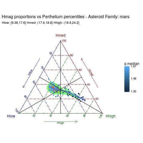
How to read the map:

• every perihelium percentile is represented by a dot
• the dot colour is associated to the median value of the perihelium percentile
• every dot has three coordinates (the sum has to be 1) representing the proportions of Hhigh, Hmed and Hlow asteroids.
• a density area is also displayed to highlight where the dots are denser
• a loess line is also drawn, though not so much significant, to give an idea of the macroscopic overall average behaviour

Note that, by definition:

• a dot near the barycenter has the same proportions of Hhigh, Hmed and Hlow (1/3+1/3+1/3).
• a dot very near to a vertex (if any) - say Hlow, it would represent a percentile where Hlow is almost equal to 1, while Hmed and High are negligible.
• a dot on a median - say the one connecting Hlow, it would represent a percentile where the High and Hmed proportions are the same.

Amor

 

IMB

 

OMB 

 

Mars Crossers

 

Trojan

 

TNO

Appendix - R script

#citation
citation();citation("reshape2");citation("ggtern");citation("ggplot2")

## 
## To cite R in publications use:
## 
##   R Core Team (2016). R: A language and environment for
##   statistical computing. R Foundation for Statistical Computing,
##   Vienna, Austria. URL https://www.R-project.org/.
## 
## A BibTeX entry for LaTeX users is
## 
##   @Manual{,
##     title = {R: A Language and Environment for Statistical Computing},
##     author = {{R Core Team}},
##     organization = {R Foundation for Statistical Computing},
##     address = {Vienna, Austria},
##     year = {2016},
##     url = {https://www.R-project.org/},
##   }
## 
## We have invested a lot of time and effort in creating R, please
## cite it when using it for data analysis. See also
## 'citation("pkgname")' for citing R packages.

## 
## To cite reshape2 in publications use:
## 
##   Hadley Wickham (2007). Reshaping Data with the reshape Package.
##   Journal of Statistical Software, 21(12), 1-20. URL
##   http://www.jstatsoft.org/v21/i12/.
## 
## A BibTeX entry for LaTeX users is
## 
##   @Article{,
##     title = {Reshaping Data with the {reshape} Package},
##     author = {Hadley Wickham},
##     journal = {Journal of Statistical Software},
##     year = {2007},
##     volume = {21},
##     number = {12},
##     pages = {1--20},
##     url = {http://www.jstatsoft.org/v21/i12/},
##   }

## 
## To cite package 'ggtern' in publications use:
## 
##   Nicholas Hamilton (2016). ggtern: An Extension to 'ggplot2', for
##   the Creation of Ternary Diagrams. R package version 2.2.0.
##   https://CRAN.R-project.org/package=ggtern
## 
## A BibTeX entry for LaTeX users is
## 
##   @Manual{,
##     title = {ggtern: An Extension to 'ggplot2', for the Creation of Ternary Diagrams},
##     author = {Nicholas Hamilton},
##     year = {2016},
##     note = {R package version 2.2.0},
##     url = {https://CRAN.R-project.org/package=ggtern},
##   }

## 
## To cite ggplot2 in publications, please use:
## 
##   H. Wickham. ggplot2: Elegant Graphics for Data Analysis.
##   Springer-Verlag New York, 2009.
## 
## A BibTeX entry for LaTeX users is
## 
##   @Book{,
##     author = {Hadley Wickham},
##     title = {ggplot2: Elegant Graphics for Data Analysis},
##     publisher = {Springer-Verlag New York},
##     year = {2009},
##     isbn = {978-0-387-98140-6},
##     url = {http://ggplot2.org},
##   }

## Loading required package: ggplot2

## --
## Consider donating at: http://ggtern.com
## Even small amounts (say $10-50) are very much appreciated!
## Remember to cite, run citation(package = 'ggtern') for further info.
## --

## 
## Attaching package: 'ggtern'

## The following objects are masked from 'package:ggplot2':
## 
##     %+%, aes, annotate, calc_element, ggplot, ggplot_build,
##     ggplot_gtable, ggplotGrob, ggsave, layer_data, theme,
##     theme_bw, theme_classic, theme_dark, theme_gray, theme_light,
##     theme_linedraw, theme_minimal, theme_void

# file name
name="apollo"
#read file
p<-read.csv(name)
# remove rows where H is not available
p<-p[which(!is.na(p$H)),]
# calculate perihelium q
p$q<-p$a*(1-p$e)
# divide H range into three equal parts
p$HT<-cut(p$H,quantile(p$H,probs=c(0,1/3,2/3,1)),include.lowest=T)
# calculate perihelium percentiles
p$qperc<-cut(p$q,quantile(p$q,probs=seq(0,1,0.01)),include.lowest=T)
# calculate q median for every q percentile
p$qm<-tapply(p$q,list(p$qperc),median)[p$qperc]
# check
head(p[,c(1,2,8,6,9:11)]);summary(p[,c(1,2,8,6,9:11)])

##          a         e         q     H          HT            qperc
## 1 1.078078 0.8268746 0.1866427 16.90 [12.4,20.8] [0.07066,0.2324]
## 2 1.245393 0.3353925 0.8276972 15.60 [12.4,20.8]  (0.8267,0.8319]
## 3 1.367258 0.4359054 0.7712628 14.23 [12.4,20.8]  (0.7681,0.7748]
## 4 1.470241 0.5599397 0.6469946 16.25 [12.4,20.8]  (0.6439,0.6558]
## 5 2.259355 0.6061736 0.8897937 15.54 [12.4,20.8]   (0.8885,0.893]
## 6 1.460856 0.6146128 0.5629953 14.85 [12.4,20.8]  (0.5582,0.5704]
##          qm
## 1 0.1835429
## 2 0.8292025
## 3 0.7709175
## 4 0.6506210
## 5 0.8904017
## 6 0.5642647

##        a                e                 q                 H        
##  Min.   : 1.000   Min.   :0.02097   Min.   :0.07066   Min.   :12.40  
##  1st Qu.: 1.294   1st Qu.:0.36393   1st Qu.:0.69437   1st Qu.:20.00  
##  Median : 1.643   Median :0.51276   Median :0.85776   Median :22.60  
##  Mean   : 1.724   Mean   :0.49672   Mean   :0.80022   Mean   :22.57  
##  3rd Qu.: 2.090   3rd Qu.:0.62793   3rd Qu.:0.95425   3rd Qu.:25.17  
##  Max.   :17.827   Max.   :0.96910   Max.   :1.01697   Max.   :33.20  
##                                                                      
##            HT                    qperc            qm        
##  [12.4,20.8]:2674   [0.07066,0.2324]:  79   Min.   :0.1835  
##  (20.8,24.4]:2621   (0.2324,0.2897] :  79   1st Qu.:0.6974  
##  (24.4,33.2]:2565   (0.3296,0.3655] :  79   Median :0.8574  
##                     (0.3981,0.4277] :  79   Mean   :0.8003  
##                     (0.4277,0.4519] :  79   3rd Qu.:0.9538  
##                     (0.4797,0.4976] :  79   Max.   :1.0160  
##                     (Other)         :7386

# build a table counting Hhigh, Hmed, Hlow in every q percentile
zz<-table(p$qm,p$HT)
# convert table so as to show proportions
zz<-zz/apply(zz,1,sum)
zz<-as.data.frame(zz)
colnames(zz)<-c("qm","hband","Freq")
zz<-dcast(zz,qm~hband)

## Using Freq as value column: use value.var to override.

colnames(zz)<-c("qm","Hlow","Hmed","Hhigh")
zz$qm<-as.numeric(as.character(zz$qm))
# check
round(head(zz),3)  

##      qm  Hlow  Hmed Hhigh
## 1 0.184 0.772 0.228 0.000
## 2 0.260 0.696 0.278 0.025
## 3 0.305 0.731 0.244 0.026
## 4 0.349 0.696 0.253 0.051
## 5 0.380 0.782 0.179 0.038
## 6 0.414 0.582 0.392 0.025

# define strings
Hlow<-paste("Hlow:",names(summary(p$HT))[1])
Hmed<-paste("Hmed:",names(summary(p$HT))[2]) 
Hhigh<-paste("Hhigh:",names(summary(p$HT))[3]) 
# plot ternary map 
myplot<-ggtern(zz,aes(Hlow,Hmed,Hhigh))
+stat_density_tern(geom='polygon',aes(fill=..level..),alpha=0.5)
+theme_rgbw()
+scale_fill_gradient(name="density",low="green",high="red",guide=F)
+geom_point(aes(col=qm))+geom_smooth_tern()
+scale_color_continuous(name="q median",breaks=round(seq(min(zz$qm),
                        max(zz$qm),length.out = 3),2),
                        limits=round(c(min(zz$qm),max(zz$qm)),2))
+ggtitle(paste("Hmag proportions vs Perihelium percentiles - Asteroid Family:",name),
         subtitle=paste(Hlow,Hmed,Hhigh))
+geom_Risoprop(value=0.5)
+geom_Lisoprop(value = 0.5)
+geom_Tisoprop(value = 0.5)