Hilda Asteroid 2017 OJ65 - an old TNO?

This object is currently an Hilda asteroid.

I run a simulation using the nominal orbital parameters read from JPL (Horizons Web Interface).

Uncertainty condition code: 0

Mercury6 simulator: configuration

More about the orbit simulator "A Hybrid Symplectic Integrator that Permits Close Encounters between Massive Bodies'' can be found here.

Main integration parameters:

   Algorithm: Bulirsch-Stoer (conservative systems)

   Integration start epoch:         2458000.5000000 days
   Integration stop  epoch:        -10^8 days
   Output interval:                     100.000 days
   Output precision:                   medium
   Initial timestep:                      0.100 days
   Accuracy parameter:             1.0000E-12
   Ejection distance:                  1.0000E+02 AU

Simulation results

This plot has been made using the R-package.

This seems to show that this asteroid was previously a TNO.

Kind Regards,
Alessandro Odasso

2016 WF9 - a simulation based on Feb 11th orbital params

This is a simulation of asteroid 2016 WF9 based on orbital parameters published on HORIZONS Web-Interface on Feb 11th, 2017.
 
At this time, the orbital condition code is 4

Orbital Elements at Epoch 2457800.5 (2017-Feb-16.0) TDB
Reference: JPL 13 (heliocentric ecliptic J2000)

Element	Value	Uncertainty (1-sigma)	Units
e	.6580360863711519	9.9808e-06
a	2.870895540801432	8.6058e-05	au
q	.9817426747520661	8.7514e-07	au
i	14.99562014245548	9.8595e-05	deg
node	125.4263986134548	0.00019086	deg
peri	342.4337260195148	8.1316e-05	deg
M	3.004319337477674	0.00013463	deg
tp	2457785.672494105614 (2017-Feb-01.17249411)	9.1832e-05	JED
period	1776.742590373345 4.86	0.07989 0.0002187	d yr
n	.2026179830159605	9.1105e-06	deg/d
Q	4.760048406850797	0.00014269	au

This asteroid was simulated with the Mercury6 orbit simulator together with 100 virtual clones generated with the package R.

These 100 clones were generated so that their orbital parameters are normally distributed around the nominal value of asteroid 2016 WF9 and their standard deviation is almost equal to the uncertainty shown above.

Virtual Asteroids: summary

	mean	sd
a	2.8709	8.68E−05
e	0.65804	9.51E−06
i	14.9956	9.48E−05
w	342.434	8.18E−05
om	125.426	0.00019
M	3.00432	0.00014

Simulation parameters

• period simulated: past 1e8 days 
• time step 0.1 days
• ejection distance = 100 au
• N-body algorithm: Conservative Bulirsch-Stoer

Simulation results

• 1 out of 101 virtual asteroid was discarded because it would have collided with Jupiter
• 44 out of 101 virtual asteroids came from the outskirt of the solar system (i.e., there was a time in the past when their distance was more than 100 au - ejection distance from the simulator point of view), so it makes sense to think they were comets.

This is the density distribution of arrival time in the solar system:

 Actually, according to the simulation, the first cometary event was 30084 years ago and the last one occurred 273009 years ago.

Probability of being a comet

I tried to use a R survival package called survminer to display the probability of a virtual asteroid being a comet, a probability that increases as you go more and more in the past.

I built a table with three columns:

• virtual asteroid id
• year: time of arrival into solar system, or end-time of the simulation (right censored data)
• event: in case of arrival from the outskirt of the solar system, this flag is TRUE, otherwise it is FALSE coherently with column year.

The Surv function available in R can be used to convert the table in order to have a formal "survival" object and the survfit function can then be used to display a summary table showing how the various asteroids were progressively lost in favor of a comet - the lost of an asteroid is equivalent to the "death" event in a survival analysis).

These are the first lines of the survfit result:

Year(in the past)	n.risk	n.event	survival	std.err	lower 95% CI	upper 95% CI
30084	101	1	0.990	0.010	0.971	1.000
67281	100	1	0.980	0.014	0.953	1.000
70233	99	1	0.970	0.017	0.938	1.000
73898	98	1	0.960	0.019	0.923	0.999
74074	97	1	0.950	0.022	0.909	0.994
75356	96	1	0.941	0.024	0.896	0.988
80292	95	1	0.931	0.025	0.882	0.982
90790	94	1	0.921	0.027	0.870	0.975

How to read:
we started with 101 virtual asteroids, then at Year 30084 in the past we see one of them coming from the outskirt of the solar system, so we do not count it as an asteroid ...then, at Year 67281 in the past, this event occurs again ... and so on till we arrive at the last virtual asteroid being counted as a comet at Year 273009 in the past (last row not shown).

Based on this, we can draw a plot showing the probability of a virtual asteroid being a comet as a function of time:

Kind Regards,
Alessandro Odasso

Citations:

Survminer
Alboukadel Kassambara and Marcin Kosinski (2016). survminer: Drawing Survival Curves using 'ggplot2'

      Mercury Simulator - Mercury6
      J.E.Chambers (1999) "A Hybrid
      Symplectic Integrator that Permits Close Encounters between
      Massive Bodies''. Monthly Notices of the Royal Astronomical
      Society, vol 304, pp793-799.

Asteroids with high perihelion precession rates

As described in this MPML message, an interesting study is under way: its goal is to
measure the perihelion precession rates for a number of objects to quantify the effects of general relativity (GR) and solar oblateness.

More at http://mel.epss.ucla.edu/jlm/research/NEAs/GR/

Based on this list, we can get the following data:

Symbol Description H Absolute magnitude a Semi-major axis (au) e Eccentricity i Inclination (deg) P Orbital period (days) SLR Semilatus rectum (au) dr Range rate due to GR/J2 (km/y) dw Perihelion shift (asec/century) arc Length of optical arc nobs Number of optical observations

Let's visually see how SLR, dr and dw are related:

• Graph 1 - dw vs SLR (parameter = quartile of dr)
  

• Graph 2 - dw vs dr (parameter = quartile of SLR) 
  

Graph 1 - dw vs SLR (parameter = quartile of dr)

> quantile of dr (km/y)
     0%     25%     50%     75%    100% 
 48.800  55.425  66.300  80.300 171.000 

Graph 2 - dw vs dr (parameter = quartile of SLR)

> quantileof SLR (au)
     0%     25%     50%     75%    100% 
0.17400 0.37400 0.48550 0.58675 0.66400

It seems to me that both graphs show (as expected) that the more an asteroid comes near the sun the more important is the dr effect.

The same is true for the dw effect but I do not understand this:

• dw belongs to an area defined by two almost linear boundaries (the slope of the higher boundary is greater than the slope of the lower boundary , thus we see a "triangular shape"...)
  Why does this happen?

Multiple regression

Coming back to easier considerations, there may be another way to show the relation between dw, dr and SLR.

Look at the multiple regression fit that predicts dw based on SLR and dr taking into
account the interaction between SLR and dr:

> summary(fit)

Call:
lm(formula = dw ~ SLR * dr, data = p)

Residuals:
     Min       1Q   Median       3Q      Max 
-2.15438 -0.30660  0.04085  0.24131  3.13628 

Coefficients:
              Estimate Std. Error t value Pr(>|t|)    
(Intercept) -27.820350   0.981042 -28.358  < 2e-16 ***
SLR          -6.124334   1.318151  -4.646 1.15e-05 ***
dr            0.146494   0.006126  23.912  < 2e-16 ***
SLR:dr        1.038595   0.028026  37.059  < 2e-16 ***
---
Signif. codes:  0 ‘***’ 0.001 ‘**’ 0.01 ‘*’ 0.05 ‘.’ 0.1 ‘ ’ 1

Residual standard error: 0.5601 on 90 degrees of freedom
Multiple R-squared:  0.9863, Adjusted R-squared:  0.9859 
F-statistic:  2163 on 3 and 90 DF,  p-value: < 2.2e-16

dw - Fitted values vs original values

This is the normal probability plot used to see how much the residuals of the model are
normally distributed:

Kind regards,
Alessandro Odasso

Near-Earth Asteroid Delta-V

JPL maintains an interesting list: Near-Earth Asteroid Delta-V for Spacecraft Rendezvous

Let's display how Delta-V depends on perihelium q=a*(1-e)

(Graphs are done with  R package and the related ggplot function)

Neo with q <=1
Delta-V (km/s) vs q (AU)

The red line is a very rough approximation for the lower boundary of Delta-V (km/s) as a function of q (AU):

delta-v = -7.3q + 11.4 when q<=1

Neo with q> 1
Delta-V (km/s) vs q (AU)

The red line is a very rough approximation for the lower boundary of Delta-V (km/s) as a function of q (AU):

delta-v = 4.6q - 0.5 when q>1

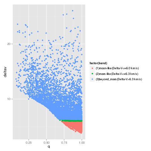
Three "bands" for Delta-V
As stated in the JPL page, for comparison, Delta-V for transferring from Low Earth Orbit to rendezvous with Moon and Mars:

• Moon: 6.0 km/s
• Mars: 6.3 km/s

Thus, we can graphically display three bands for Delta-V. I call them as follows:
1) moon-like (Delta-V <= 6.0 km/s)
2) mars-like (Delta-V <= 6.3 km/s)
3) beyond-mars (Delta-V > 6.3 km/s)

Neo with q <=1
Delta-V (km/s) vs q (AU)

Neo with q > 1

Delta-V (km/s) vs q (AU)

We can look at the neo distribution in every Delta-V band:

Neo with q <=1

Neo with q >1

Ultra-low Delta-V Neo

I often read that these neo are considered as a particular interesting target for   spacecraft rendezvous missions because very little energy is needed to reach them.

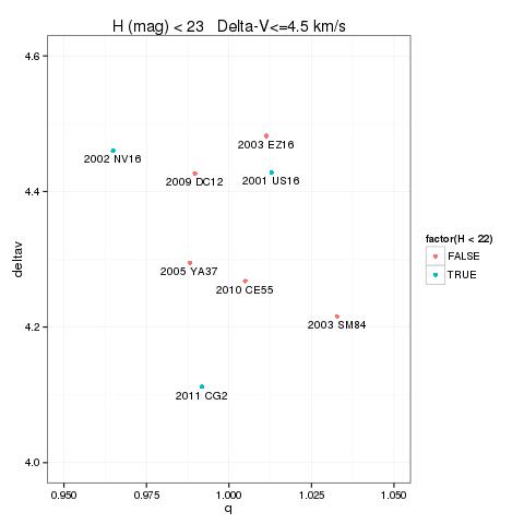
This is a graphical display for neo with Delta-V <= 4.5 km/s:

These ultra low Delta-V neo are just a tiny fraction of the neo population.
This is their proportion:

As known, one of the problems with these neo is that it is very difficult to find relative bright (and thus big) asteroids.

The graph below shows all the ultra low Delta-V asteroids with H (mag) <= 23 showing that only three neo of this group have H (mag) <= 22. They are:

Designation	Delta-V (km/s)	H (mag)
2011 CG2	4.112	21.5
2001 US16	4.428	20.2
2002 NV16	4.460	21.4

(1999 RQ36) Bennu and ("similar?") Neo

Delta-V for Bennu: 5.087 km/s
H (mag) = 20.9

See also:
http://en.wikipedia.org/wiki/101955_Bennu
http://astro.mff.cuni.cz/davok/papers/bennu_osiris_maps2015.pdf

If we give a look at asteroids having Delta-V and H at least comparable (or better) than those of asteroid Bennu, target of the OSIRIS-REx mission, we can find a few other ones.
Bennu is shown at the top-left corner of the image.

Of course, Delta-V is not the only parameter used to decide whether an asteroid is a good candidate for a sample return mission (physical characteristics, a well known orbit and an appropriate rendezvous time are certainly other fundamental aspects!). 

Once said this, I would be interested to know if some of the other asteroids shown here are candidates for similar missions.
In fact, I found an interesting link showing the earth-centric orbit view of many of these asteroids

 

Kind Regards,
Alessandro Odasso