astro: 2011 DL12 = K11D12L -- Cometary Origin?

2011 DL12 is an outer main-belt asteroid.

I have downloaded the orbital parameters from JPL Small-Body Database Browser:

[ show orbit diagram ]

Orbital Elements at Epoch 2458600.5 (2019-Apr-27.0) TDB
Reference: JPL 4 (heliocentric ecliptic J2000)

Element	Value	Uncertainty (1-sigma)	Units
e	.3332919522378502	1.7048e-05
a	3.813848977356317	0.00010804	au
q	2.542723806152901	1.7234e-05	au
i	13.48245115796516	0.00011571	deg
node	329.3312783932701	0.00010623	deg
peri	151.9591228706485	0.0023481	deg
M	48.29805632413862	0.016968	deg
t_p	2458235.518528997214 (2018-Apr-27.01852900)	0.11275	TDB
period	2720.468266449358 7.45	0.1156 0.0003165	d yr
n	.1323301596419123	5.6232e-06	deg/d
Q	5.084974148559733	0.00014405	au

Orbit Determination Parameters

# obs. used (total)	22
data-arc span	413 days (1.13 yr)
first obs. used	2010-01-15
last obs. used	2011-03-04
planetary ephem.	DE431
SB-pert. ephem.	SB431-N16
condition code	4
fit RMS	.85076
data source	ORB
producer	Otto Matic
solution date	2018-Oct-18 05:08:18

Additional Information

Earth MOID = 1.56728 au

Jupiter MOID = .136519 au

T_jup = 2.934

(2011 DL12)

Classification: Outer Main-belt Asteroid SPK-ID: 3558704

I generated 100 clones trying to achieve the same nominal orbital parameters and uncertainty as calculated by JPL.

The result (achieved vs target) is shown in this table:

	Clones		Target
	mean	sd	mean	sd
q	2.54272169	1.715e-05	2.54272381	1.723e-05
e	0.33329091	1.712e-05	0.33329195	1.705e-05
i	13.48245868	0.00011564	13.48245116	0.00011571
peri	151.95937755	0.00234384	151.95912287	0.0023481
node	329.33127117	0.00010601	329.33127839	0.00010623
tp	2458235.53032508	0.11307094	2458235.518529	0.11275

Backward Simulation

As shown below, I investigated what could have happened to the clones in the past going back to -100 million JD (about 280K years in the past).

As arbitrary threshold to declare that an object is likely to have a cometary origin, I set ejection distance = 100 AU

Algorithm: Bulirsch-Stoer

Non gravitational effects: not taken ito account.

Software: Mercury 6

===> reference for the package: J.E.Chambers (1999) ``A Hybrid
      Symplectic Integrator that Permits Close Encounters between
      Massive Bodies''. Monthly Notices of the Royal Astronomical
      Society, vol 304, pp793-799.

)O+_06 Integration parameters (WARNING: Do not delete this line!!)
) Lines beginning with `)' are ignored.
)---------------------------------------------------------------------
) Important integration parameters:
)---------------------------------------------------------------------
algorithm (MVS, BS, BS2, RADAU, HYBRID etc) = BS
start time (days)= 2458200.5
stop time (days) = -1d8
output interval (days) = 100
timestep (days) = 0.05
accuracy parameter=1.d-12
...
ejection distance (AU)= 100

Simulation Results

(all analysis and plots below are done with R version 3.5.1 (R: A Language and Environment for Statistical Computing) using many libraries including library ggplot and viridis).

Going back in the past, 77 out of 100 clones seem to have a cometary origin because they entered the solar system coming from a distance greater than 100 AU.

As the simulation is backward, this plot should be read from right to left: we can see that many of the initial 100 clones are slowly "ejected" from the solar system (i.e. they entered in the solar system):

This plot show the density distribution of the arrival time in the solar system:

It seems that the most of the clones arrived in the solar sytem about 35000 years ago.

Footprint plots

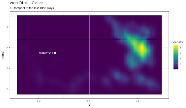
If we forget the temporal dimension, we can draw some "footprint" plots that show where the clones were for most of the time:

Time plots

In the following plots, we take again into consideration the temporal dimension.

We start defining 10 time slots.
We take the first time slot and consider the first clone: we calculate the mean (or min/max) of an orbital parameter. Thus, we have one value.

Then, we do the same calculation for the other clones in the first time slot and we draw the resulting boxplot showing the distribution of all values.

The number of clones contributing to each interval in written over the boxplot itself.
The process is repeated for every time slot.

minimum value of perihelium

In case of aphelium, we need to discard a couple of outliers in order to be able to see the boxplots that otherwise would be too much "compressed":

maximum value of aphelium

maximum value of eccentricity:

mean value of inclination

mean value of w

mean value of om

In the energy plot, clones with hyperbolic orbits have energy greater than 0

maximum value of energy

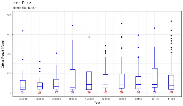
For hyperbolic clones we can show the Vinfinity while for the other we can show the orbital period (in the latter case, we discard a few outliers to better see the boxplots):

maximum value of Vinfinity